The I-Eval is used to enhance the basic analyzing feature into a flexible and
comprehensive image manipulator for dedicated goals. It serves as a replacement for
writing a dedicated code (in your favorite HL/script language) or for quick image
manipulating that can further complement the analyzing procedure.
The main functionality of the I-Eval is iterating an image(s) pixels in raster order and
allowing to output any value in order to create a new 1/3 channels (components) image.
This is achieved by writing a c-like expression that is iterated per pixel with the proper
context. You can use it to swap channels data, transform an image, mask, average and
anything that can cross your mind.
For the benefit of clarity, all noted expressions will be enclosed with {…} which is
non-mandatory if you wish to apply single expression (refer to multi I-Eval notes).
The best way to understand its usage is by examples:
Suppose you have a comparison party of 2 gray images and the regular diff action is too
“binary” for your task and you need it to count as difference only if the delta is
larger than 4, for this you will write:
{ (abs(i2-i1) > 4)*255 }
Suppose you have now RGB image with the same problem and you wish to create a single
diff image, then:
{ (abs(i2c1-i1c1) > 2 || abs(i2c2-i1c2) > 2 || abs(i2c3-i1c3) > 2)*255 }
Note that because the input is 3-channels, you must select the ‘Forced single’ option else
you will get a 3 channels output (on that further).
Base syntax and guidelines:
- You can use I-Eval on single image or on a comparison party. When in compare mode, the
images are ordered 1 to N (left to right, visual order). - You refer to an image with ‘i’+#. ‘i’ alone is the same as i1. If you wish to
differentiate the channels, you can add the ‘c’+# (1..3) syntax. ‘c’ alone refers to i1
by context (so if you have a 3 ch. image and you’re on ch. 2 then it’s the same as
writing explicitly i1c2). - You can give different expression per channel via ‘;’. Even if the input is of 1 ch.,
you can create an output of 3 ch. by writing expression like {c;c;c}. If you write an
expression like { (i2+i1)/2; abs(i2-i1); i2^2/i1^2 } then the I-Eval engine will apply
the proper value per channel so the above is equivalent to the expanded expression:{ (i2c1+i1c1)/2; abs(i2c2-i1c2); i2c3^2/i1c3^2 } - You can mix 1 ch. and 3 ch. images in the same expression as the engine will match the
proper channel semantics. However, writing token like i2c2 for a 1 ch. image will have
a don’t care affect (as if it was i2c1). - To allow strong expressions, ‘x‘ and ‘y‘ are reserved variables that state the currently
iterated coordinate. This is useful to distinguish the spatial location in a run like
masking only odd lines with { (y % 2)*i }. Note that the coordinate is 0-based so we
start at <0,0> and end at <w-1,h-1>. - You can also use ‘w‘ and ‘h‘ to state width and height which is quite useful for say,
mirroring an image horizontally {c[w-1-x,y]} or vertically {c[x,h-1-y]}. - When ROI in an image is active, you can use in the expression the following variables:
x1,y1,x2,y2,cw,ch which means respectively: left, top, right, bottom, crop area width
and crop area height. - You can access at any iteration any required pixel by using the indexing syntax of
i[X,Y] (or c[X,Y], i2c3[X,Y], etc.). This is super important if you wish to apply any
kind of transform or kernel based filter. A simple 3×3 dilate operation can be:{ ((c[x-1,y-1]+c[x,y-1]+c[x+1,y-1]+c[x-1,y]+c+c[x+1,y]+c[x-1,y+1]+c[x,y+1]+ c[x+1,y+1]) > 0) * 255 } - The indexing feature supports any dereferencing level so if you have 2 images that one
is used as a distance seed map, you can write expression like {i[i2[x,y],i2[x*2,y*2]]}.
See the dialog options section for ‘out-of-range values’. - If in some dereference context, X or Y are not positive integer (0 included) then
a truncated value will be used. - If you wish to apply several operations in a pipe fashion, you can write several I-Eval
expressions with this basic syntax {…} {…}. Good example is Opening (erode+dilate)
that can be achieved by (for 3×3 kernel):{ ((c[x-1,y-1]+c[x,y-1]+c[x+1,y-1]+c[x-1,y]+c+c[x+1,y]+c[x-1,y+1]+c[x,y+1] +c[x+1,y+1]) > 0) * 255 } { ((c[x-1,y-1]+c[x,y-1]+c[x+1,y-1]+c[x-1,y]+c+c[x+1,y] +c[x-1,y+1]+c[x,y+1]+c[x+1,y+1]) == 255*9) * 255 } - As expressions can be complex, you can save them for later usage and apply them via
the ‘List of saved I-Eval expressions’ list. Each L-double-click will append the
selected I-Eval to the currently edited expression. Use R-click to expand the I-Eval
expression itself (good for temporary editing). - You can reference a saved expression via $saved name$ (must be a complete I-Eval
expression) so the above example, assuming you saved Erode3x3 and Dilate3x3 can be
entered as {$Erode3x3$} {$Dilate3x3$}. You can further optimize your work by declaring
a new I-Eval named Opening_3x3 as {$Erode3x3$} {$Dilate3x3$} and place $Opening_3x3$
in the editor. - An I-Eval name must start with a [a-z,A-Z,_] and can be followed by alpha-numeric and
any of ‘ :;,-+*/=~_&|#!?(){}[]’. - All expressions are case sensitive.
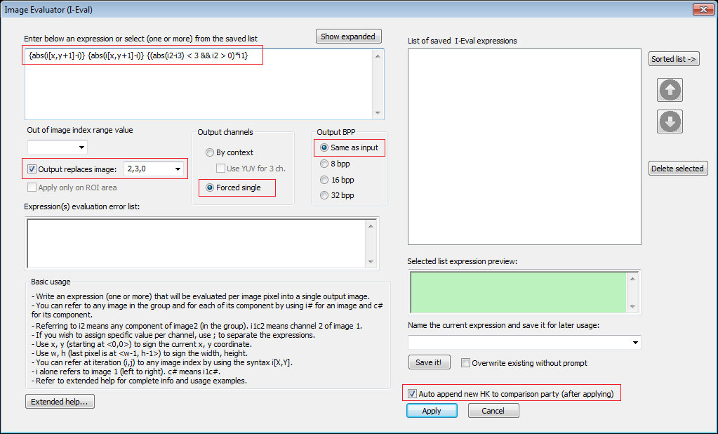
Dialog GUI options (I-Eval control parameters)
- Out of image index range value
If you use expression like i2[x-20,y] then it’s obvious that for the 20 first
iterations in each row, you will point to index in the image that isn’t legit. For
that, you can supply a value (or per channel by using ‘;’) that will be auto-set
whenever the offset in the image goes out-of-range. Default is 0. - Output replaces image
By default, a new image will be created as an output, appended in a new valid HK.
You may, however, wish to replace one of the inputs (done at iteration end, not
in-place so input is persistent) so you just enter here an index (1..N) while empty
or 0 state a new HK. When you invoke several I-Eval expressions in a pipe, you may
wish to direct each intermediate image evaluation to a different output so if you
have, let’s say, 3 consecutive I-Eval and 4 input images, you may write ‘2,1,3’ so
after the first I-Eval, image 2 will be replaced with the output and so on. If you
supply less indexes than the no. of I-Eval, then the last is appended to fill the
gap (i.e. for the above example, ‘2,1’ is the same as ‘2,1,1’). You can assign 0 as
a last entry to state a new image output (recall you can’t access it in intermediate
operations as it’s not part of the comparison party).
Note that you can’t change input image no. of channels when using piped I-Eval i.e.
if you wish to output over image 2 but your expression presume 1 ch. data then it
will raise a parse error or simply duplicate the channels. - Apply only on ROI area
In case there’s an active ROI, you can choose to apply the I-Eval on its region
which can help reducing evaluation time and even yield smart scale/morph image
manipulations. - Output channels
Supported raw images have 1 or 3 channels (components). As such, you may influence
the I-Eval no. of output channels. If you select ‘By context’ then you wish that
the engine will analyze the input expression and if the input image has 1 ch. then
the output will have 1. If the input has 3 ch. then the output will have 3. If the
expression holds per-channel expression (like {i;i;i}) then you wish to create 3 ch.
output. All 3 channels output are formatted as planner RGB by default unless the
“Use YUV for 3 ch.” is checked.
Still, there are cases where the input is holding 3 ch. but you wish to evaluate a
single channel output, for those cases, you should select the ‘Forced single’.
Note that trying to force a single output on a 3 comp. expression is considered an
error. - Output BPP
You can control the BPP (bits-per-pixel/bits-depth) of the output image. This is very
useful when you wish to expand or reduce (quantize) an image datum. Selecting auto
will use image 1 as anchor (and thus forcing all others to align with it, no matter
their actual BPP). Quick example is gradient image: Suppose you have 8 BPP luma image
and you wish to create a gradient image for the x axis (frequency domain), then
{ i[x+1,y]-i } should give that but a negative value like (6-100 = -94) will be
clipped to 0 so if the output is 16 BPP you can write something like
{i[x+1,y]-i + 255} and all values will range [0,510]. - Expression(s) evaluation error list
As its name states, here you will see a report for input or evaluation errors that
might occur due to complexity of the entered expressions (syntax, math errors, etc.). - List of saved I-Eval expressions
This serves as a pseudo-macro generator. Many expressions are very complex and instead
of saving them in your favorite text editor, you can save them here and give them a
proper name. You may save here even piped expressions ({…} {…} …).
Suppose you have an image quantizer expression like {(i+2^4) >> 5} so a good name
might be ‘3bit Quantizer’ and so on.
Note that each double-click (select) on a list item will concatenate it to the
currently edited I-Eval expression with a {$I-Eval name$} markup. R-click on a
selected name will put the I-Eval expression itself {…} so you may edit it before
submission. If you save over an existing name and overwrite w/o prompt isn’t checked,
you’ll be prompted to overwrite it. Use ‘Delete selected’ to delete unused items.
You can save the same expression with different names, it’s completely a user’s
choice.
All saved expressions are saved under ‘ria.ieval.txt’ (default, see Config file) in
plain text form with <name> … </name> style. Feel free to modify it outside if more
convenient. - Sorted list / Custom list
To assist the saved I-Eval list organization, you can choose to view the items in
sorted or custom order.
The custom (default, the button will show switch to “Sorted list”) allows you to
set the data as you see fit and you can use the Up/Down arrow buttons to customize a
different layout and, for an example, put more frequently used items higher or by
pseudo-logical groups.
The sorted (the button will show switch to “Custom list”) allows you to view the
list in lexicographic (A-Z) order. Do note you can’t edit the list order (obvious, as
it’s sorted…).
One note regarding the file that stores the list – it always reflects the custom
order so you can easily manipulate it with an external editor by your choice. - Expanded / Original expression
For complex expressions, if the parser reported some error or you wish to see expanded
nested expressions, toggle between this views to fine-tune your edited I-Eval or
pin-point a parsing error.
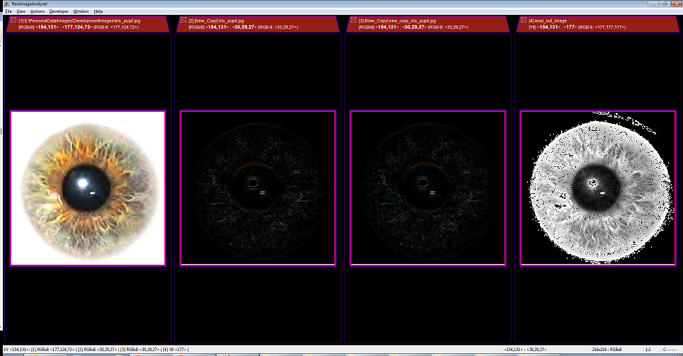
Example that shows how to create X,Y gradients and then use these 2 gradient images
as a mean to create a luma mask of the original image (in our case, that the 2 gradients
are close to one another)
Expression strength
- The expression can be written in a c-like form while incorporating many standard math
and logic functions / operands. All follow standard operator precedence. - Any intermediate calculation is done on 64b values, may them be DP (double) or
integer. This requires extra clarification: No matter the images (or selected)
bits-depth, you are assured all intermediate calculations are performed with max
flexibility and only in the end, the values are clipped to their proper BPP limits. - The final value is always clipped to the output BPP range and any DP values are
truncated (and not rounded so use round(x) if you require a rounded value). - The math constants e (2.71…) and pi (3.14…) are a 64b constant variables.
- Functions that have domain constraints, will raise an error for invalid input.
- You can use 0xNNNN to sign hexa-decimal numbers (0x1F) and NNNNb to sign bin (101b).
| Logic operands | Output yields 0/1 |
|---|---|
| || | Or |
| && | And |
| ! | Not |
| Comparison operands | Output yields 0/1 |
| < | Lower than |
| > | Greater than |
| <= | Lower than or equal |
| >= | Greater than or equal |
| == | Equal |
| != | Not equal |
| Bitwise operands | Integer only |
| & | And |
| | | Or |
| ~ | Complement |
| |^ | Xor |
| >> | Shift right, signed |
| << | Shift left |
| Basic algebra | |
| + | Addition |
| – | Subtraction |
| * | Multiplication |
| / | Division Note it’s context aware i.e. if the expression is integer then it will use an integer divider (like truncation) else the floating-point one |
| ^ | Power of (63, 4-(1/3), …) |
| % | Integer modulo, iso-c semantics |
| Trigonometric | Input is in radians unless stated otherwise |
| sin(x) | Sine |
| cos(x) | Cosine |
| tan(x) | Tangent |
| atan2(y,x) | Arctangent (by quadrant) |
| rad(x) | Radian of 360 deg. angle |
| deg(x) | Degree (-2Π.. 2Π) |
| General math | |
| sign(x) | Return -1 if x < 0, +1 if x > 0, else 0 |
| exp(x) | Same as ex. Choose your flavor |
| log(x) | Natural logarithm (e) |
| log10(x) | Decimal-base (10) logarithm |
| logb(b,x) | B-base logarithm (e.g logb(2,8) = 3) |
| abs(x) | Absolute value of x (noted |x|) |
| sqrt(x) | Square-root. Same as x0.5 but uses a dedicated function. |
| dist(x,y) | Distance of <x,y> from <0,0>. Named radius in polar coordinates |
| max(a,b) | Maximum of a and b |
| min(a,b) | Minimum of a and b |
| bits(x) | No. of bits required to represent |x|. Can be float but reflects only the integer part |
| Integer only in/out | |
| bool(x) | Evaluate x to be either 1 (if not 0) or 0 |
| fact(x) | Factorial of x (x!). Bounded by 64b val |
| binom(k,n) | Binomial coefficient (same as k-selection) |
| Conversion | |
| floor(x) | Rounds x downward. Result is integer. E.g floor(3.2) = 3, floor(-5.1) = -6 |
| ceil(x) | Rounds x upward. Result is integer. E.g ceil(3.2) = 4, ceil(-5.1) = -5 |
| round(x) | Rounds x. Result is integer. E.g round(3.2) = 3, round(-5.1) = -5, round(-5.6) = -6 |
| double(x) | Converts x to double. Useful for division (3/double(x), while x = 2) |
The best way to understand how I-Eval can be useful is by several common examples.
Example 1
Blending 2 images while image 3 serves as alpha map (assuming 8bpp values).
round((i3*i1 + i2*(255-i3))/255.0)
Example 2
Put image 1 over image 2 if image 2 values are below a threshold of 5.
(i2 >= 5)*i1 + (i2 < 5)*i2
Example 3
The famous fish-eye effect in a center of image, radius of 100 and curvature factor
of 0.01. Let’s assume the image is at least 100×100. The rest remains as is. The general
way to do it is using polar coordinates transform and defining some smooth factor (s)
as ‘rad/log(curvFactor*rad+1)’ so the new radius becomes ‘(e^(rad/s)-1)/curvFactor’,
expanding all yields:
   (dist(x-w/2, y-h/2) <= 100)*i[
   w/2+cos(atan2(y-h/2,x-w/2))*(exp(dist(x-w/2, y-h/2)/(100/(log(100*0.01+1))))-1)/0.01,
   h/2+sin(atan2(y-h/2,x-w/2))*(exp(dist(x-w/2, y-h/2)/(100/(log(100*0.01+1))))-1)/0.01]+
   (dist(x-w/2, y-h/2) > 100)*i
Note that if you use it in several scenarios, you can use macros and make it more
readable (like ang = atan2(y-h/2,x-w/2)).
Example 4
Apply white-balance and black level. We assume the WB value is 220 and BL is 15.
round(i*(255.0/220))+15
Example 5
Making a mask of a key-color value range (say 4..8).
255*(i >= 4 && i <= 8)
Example 6
Simple 3×3 averaging-like kernel-based filter (rounded final value).
    round((c[x-1,y-1]*1+c[x,y-1]*2+c[x+1,y-1]*1+
    c[x-1,y]  *1+c       *3+c[x+1,y]  *1 +
    c[x-1,y+1]*1+c[x,y+1]*2+c[x+1,y+1]*1)/14.0)
Example 7
Using the pipe feature to create a gradient X and Y images. We assume we have 3 images
in the group and only image 1 is immutable and our output overwrite sequence will be
2,3 and output is 16bpp (input is gray-8bpp, 2, 3 are gray-16bpp).
{i[x+1,y]-i + 255} {i[x,y+1]-i + 255}
If you wish to see the visual outcome of the gradients, you can try the following in
order to “stretch” the 16b values:
{(i[x+1,y]-i + 255) << 7} {(i[x,y+1]-i + 255) << 7}
Example 8
Converting RGB into HSV model. In our example we’ll calculate Hue, Chroma and Value
(a.k.a M) respectively. (R,G,B) = (c1,c2,c3)
   atan2(0.5*sqrt(3)*(c2-c3), 0.5*(2*c1-c2-c3)) ;
   dist(0.5*(2*c1-c2-c3), 0.5*sqrt(3)*(c2-c3))  ;
   max(max(c1, c2), c3)
Note that this will yield HSV values while the visual side-effect will be undefined.
Example 9
Simple image rotation around the center by 30 deg. (invalid areas will be black).
i[w/2+(x-w/2)*cos(pi/6) - (y-h/2)*sin(pi/6), h/2+(x-w/2)*sin(pi/6) + (y-h/2)*cos(pi/6)]
Example 10
Creating a cropped (no interpolation) Bayer RGGB image. Output is forced 1.
   (x % 2 == 0 && y % 2 == 0)*c1 +
   ((x % 2 == 1 && y % 2 == 0) || (x % 2 == 0 && y % 2 == 1))*c2 +
   (x % 2 == 1 && y % 2 == 1)*c3
Example 11
Converting Bayer RGGB to RGB. Very useful for sensor raw images.
   (x % 2 == 0 && y % 2 == 0)*i + (x % 2 == 1 && y % 2 == 0)*(i[x-1,y] + i[x+1,y])/2 +
   (x % 2 == 0 && y % 2 == 1)*(i[x,y-1] + i[x,y+1])/2 +
   (x % 2 == 1 && y % 2 == 1)*(i[x-1,y-1] + i[x+1,y-1] + i[x-1,y+1] + i[x+1,y+1])/4 ;
   ((x % 2 == 0 && y % 2 == 0) || (x % 2 == 1 && y % 2 == 1))*(i[x-1,y] + i[x+1,y])/2 +
   ((x % 2 == 1 && y % 2 == 0) || (x % 2 == 0 && y % 2 == 1))*i ;
   (x % 2 == 0 && y % 2 == 0)*(i[x-1,y-1] + i[x+1,y-1] + i[x-1,y+1] + i[x+1,y+1])/4 +
   (x % 2 == 1 && y % 2 == 0)*(i[x,y-1] + i[x,y+1])/2 + (x % 2 == 0 && y % 2 == 1)*
   (i[x-1,y] + i[x+1,y])/2 + (x % 2 == 1 && y % 2 == 1)*i
Obviously, this expanded expression is a bit hard to follow so a good approach will be
to define the 4 Bayer pixels (and operands) as:
   p00 = (x % 2 == 0 && y % 2 == 0)
   p01 = (x % 2 == 1 && y % 2 == 0)
   p10 = (x % 2 == 0 && y % 2 == 1)
   p11 = (x % 2 == 1 && y % 2 == 1)
   avrLR = (i[x-1,y] + i[x+1,y])/2
   avrTB = (i[x,y-1] + i[x,y+1])/2
   avrD4 = (i[x-1,y-1] + i[x+1,y-1] + i[x-1,y+1] + i[x+1,y+1])/4
So the above long expression can be written as:
   $p00$*i + $p01$*$avrLR$ + $p10$*$avrTB$ + $p11$*$avrD4$ ;
   ($p00$ || $p11$)*$avrLR$ + ($p01$ || $p10$)*i ;
   $p00$*$avrD4$ + $p01$*$avrTB$ + $p10$*$avrLR$ + $p11$*i
By using these 7 macros, you can easily define any Bayer sub-pattern.
Example 12
Image negative. Same as CMY (suits both 1/3 channels image).
255-i
Example 13
Simple downscale by a factor of 2 with bi-linear interpolation. We assume there’s an
active ROI from <0,0> with size (w/2)x(h/2) and that we’re working solely on the ROI
area.
(i[x*2,y*2] + i[x*2+1,y*2] + i[x*2,y*2+1] + i[x*2+1,y*2+1])/4
Example 14:
This will demo a very complex example of applying the Zhang-Suen thinning algorithm on
binary (or luma-based images). As the algorithm is iterative, we’ll create several
macros to assist us in the process. Recall you can edit by yourself the I-Eval saved
expressions file so let’s assume we have there (p2 above center point, going CW):
p2 = (c[x,y-1] != 0), p3 = (c[x+1,y-1] != 0), ..., p9 = (c[x-1,y-1] != 0)
Now we can use them as macro-blocks and create 2 iterations:
   ZSAlg_A =
        ($p2$ == 0 && $p3$ == 1) + ($p3$ == 0 && $p4$ == 1) +
        ($p4$ == 0 && $p5$ == 1) + ($p5$ == 0 && $p6$ == 1) +
        ($p6$ == 0 && $p7$ == 1) + ($p7$ == 0 && $p8$ == 1) +
        ($p8$ == 0 && $p9$ == 1) + ($p9$ == 0 && $p2$ == 1)
   ZSAlg_B = $p2$ + $p3$ + $p4$ + $p5$ + $p6$ + $p7$ + $p8$ + $p9$

   ZSAlg_iter0_m1 = ($p2$ * $p4$ * $p6$)
   ZSAlg_iter1_m1 = ($p2$ * $p4$ * $p8$)
   ZSAlg_iter0_m2 = ($p4$ * $p6$ * $p8$)
   ZSAlg_iter1_m2 = ($p2$ * $p6$ * $p8$)

   ZSAlg_iter0_marker =
        ($ZSAlg_A$ == 1 && ($ZSAlg_B$ >= 2 && $ZSAlg_B$ <= 6) &&
        $ZSAlg_iter0_m1$ == 0 && $ZSAlg_iter0_m2$ == 0)*255
   ZSAlg_iter1_marker
        ($ZSAlg_A$ == 1 && ($ZSAlg_B$ >= 2 && $ZSAlg_B$ <= 6) &&
        $ZSAlg_iter1_m1$ == 0 && $ZSAlg_iter1_m2$ == 0)*255
We’ll define the mask while assuming it’s referring to image 2
ZSAlg_marker_mask = 0*(i2 != 0)+i*(i2 == 0)
Now, the final single iteration will be consisted of the above 3 building blocks:
   ZSAlg_iter =
        {$ZSAlg_iter0_marker$} {$ZSAlg_marker_mask$}
        {$ZSAlg_iter1_marker$} {$ZSAlg_marker_mask$}
All we need is to duplicate our source image using <n>, enter comparison mode, put
$ZSAlg_iter$ as I-Eval and set the output replace sequence to be 2,1,2,1 and we got
ourself a mean to inspect a single iteration of this nice thinning algorithm.
Later, using Ctrl-[E], you can further iterate the algorithm steps until reaching a
non-changing image. You can create 2 copies of your original image and put the original
as a 3rd panel and see how it changes progressively (or create a diff image and monitor
the thinning steps).
Minor notes regarding the evaluation process:
As processing complex expressions is very exhaustive (cpu-wise), several optimizations
are done in order to evaluate it faster. You should know that the expression is being
pseudo-compiled into a lower level notation and that redundancies in calculation are
omitted by pre-evaluation of constant values and caching of already evaluated values.